File System Management

File-System Layout

File Systems are stored on disks. The above figure depicts a possible File-System Layout.

• MBR: Master Boot Record is used to boot the computer
• Partition Table: Partition table is present at the end of MBR. This table gives the starting and ending addresses of each partition.
• Boot Block: When the computer is booted, the BIOS reads in and executes the MBR. The first thing the MBR program does is locate the active partition, read in its first block, which is called the boot block, and execute it. The program in the boot block loads the operating system contained in that partition. Every partition contains a boot block at the beginning though it does not contain a bootable operating system.
• Super Block: It contains all the key parameters about the file system and is read into memory when the computer is booted or the file system is first touched.

Implementing Files

Contiguous Allocation: Each file is stored as a contiguous run of disk blocks. Example: On a disk with 1KB blocks, a 50KB file would be allocated 50 consecutive blocks. With 2KB blocks it would be 25 consecutive blocks.

Advantages:

Simple to implement.

The read performance is excellent because the entire file can be read from the disk in a single operation.

Drawbacks:

Over the course of time the disk becomes fragmented.

Linked List Allocation:

The second method for storing files is to keep each one as a linked list of disk blocks. The first word of each block is used as a pointer to the next one. The rest of the block is for data. Unlike Contiguous allocation no space is lost in disk fragmentation.

Layered File System

I/O control:: device drivers and interrupt service routines that perform the actual block transfers.

Basic file system:: issues generic low-level commands to device drivers.

File organization:: translates logical block addresses to physical block addresses.

Logical-file-system::Handles metadata that includes filesystem  structure (e.g., directory structure and file control blocks (FCB’s)

Virtual File Systems:

An operating system can have multiple file systems in it. Virtual File Systems are used to integrate multiple file systems into an orderly structure. The key idea is to abstract out that part of the file system that is common to all file systems and put that code in a separate layer that calls the underlying concrete file system to actually manage the data.

Structure of Virtual File Systems in UNIX system:

The VFS also has a 'lower' interface to the concrete file systems, which is labeled VFS interface. This interface consists of several dozen function calls that the VFS can make to each file system to get work done. VFS has two distinct interfaces: the upper one to the user processes and the lower one to the concrete file systems VFS supports remote file systems using the NFS (Network File System) protocol.

File Access Methods

Let's look at various ways to access files stored in secondary memory.

1. Sequential Access:
2. Direct Access:
3. Indexed Access:

1.Sequential Access:

Most of the operating systems access the file sequentially. In other words, we can say that most of the files need to be accessed sequentially by the operating system.In sequential access, the OS read the file word by word. A pointer is maintained which initially points to the base address of the file. If the user wants to read first word of the file then the pointer provides that word to the user and increases its value by 1 word. This process continues till the end of the file, due to the fact that most of the files such as text files, audio files, video files, etc need to be sequentially accessed

2.Direct Access:

The Direct Access is mostly required in the case of database systems. In most of the cases, we need filtered information from the database. The sequential access can be very slow and inefficient in such cases.Suppose every block of the storage stores 4 records and we know that the record we needed is stored in 10th block. In that case, the sequential access will not be implemented because it will traverse all the blocks in order to access the needed record.

Direct access will give the required result despite of the fact that the operating system has to perform some complex tasks such as determining the desired block number. However, that is generally implemented in database applications.

3.Indexed Access:

If a file can be sorted on any of the filed then an index can be assigned to a group of certain records. However, A particular record can be accessed by its index. The index is nothing but the address of a record in the file.

In index accessing, searching in a large database became very quick and easy but we need to have some extra space in the memory to store the index value.

Directory

        Directory can be defined as the listing of the related files on the disk. The directory may store some or the entire file attributes.To get the benefit of different file systems on the different operating systems, A hard disk can be divided into the number of partitions of different sizes. The partitions are also called volumes or mini disks. Each partition must have at least one directory in which, all the files of the partition can be listed. A directory entry is maintained for each file in the directory which stores all the information related to that file.

          A directory can be viewed as a file which contains the Meta data of the bunch of files.Every Directory supports a number of common operations on the file:

1.   File Creation

2.   Search for the file

3.   File deletion

4.   Renaming the file

5.   Traversing Files

6.   Listing of files

Single Level Directory

The simplest method is to have one big list of all the files on the disk. The entire system will contain only one directory which is supposed to mention all the files present in the file system. The directory contains one entry per each file present on the file system.

This type of directories can be used for a simple system.

Advantages

1.   Implementation is very simple.

2.   If the sizes of the files are very small then the searching becomes faster.

3.   File creation, searching, deletion is very simple since we have only one directory.

Disadvantages

1.   We cannot have two files with the same name.

2. The directory may be very big therefore searching for a file may take so much time.

3.   Protection cannot be implemented for multiple users.

4.   There are no ways to group same kind of files.

5. Choosing the unique name for every file is a bit complex and limits the number of files in the system because most of the Operating System limits the number of characters used to construct the file name.

Two Level Directory

In two level directory systems, we can create a separate directory for each user. There is one master directory which contains separate directories dedicated to each user. For each user, there is a different directory present at the second level, containing group of user's file. The system doesn't let a user to enter in the other user's directory without permission.

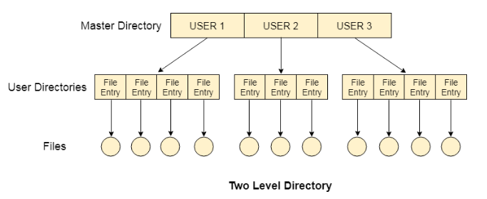
Characteristics of two level directory system

1.   Each files has a path name as /User-name/directory-name/

2.   Different users can have the same file name.

3.   Searching becomes more efficient as only one user's list needs to be traversed.

4.   The same kind of files cannot be grouped into a single directory for a particular user.

Every Operating System maintains a variable as PWD which contains the present directory name (present user name) so that the searching can be done appropriately.

Tree Structured Directory

In Tree structured directory system, any directory entry can either be a file or sub directory. Tree structured directory system overcomes the drawbacks of two level directory system. The similar kind of files can now be grouped in one directory.

Each user has its own directory and it cannot enter in the other user's directory. However, the user has the permission to read the root's data but he cannot write or modify this. Only administrator of the system has the complete access of root directory.

Searching is more efficient in this directory structure. The concept of current working directory is used. A file can be accessed by two types of path, either relative or absolute.Absolute path is the path of the file with respect to the root directory of the system while relative path is the path with respect to the current working directory of the system. In tree structured directory systems, the user is given the privilege to create the files as well as directories

Permissions on the file and directory

A tree structured directory system may consist of various levels therefore there is a set of permissions assigned to each file and directory.

The permissions are R W X which are regarding reading, writing and the execution of the files or directory. The permissions are assigned to three types of users: owner, group and others.

There is a identification bit which differentiate between directory and file. For a directory, it is d and for a file, it is dot (.)

The following snapshot shows the permissions assigned to a file in a Linux based system. Initial bit d represents that it is a directory.

Acyclic-Graph Structured Directories

The tree structured directory system doesn't allow the same file to exist in multiple directories therefore sharing is major concern in tree structured directory system. We can provide sharing by making the directory an acyclic graph. In this system, two or more directory entry can point to the same file or sub directory. That file or sub directory is shared between the two directory entries.

These kinds of directory graphs can be made using links or aliases. We can have multiple paths for a same file. Links can either be symbolic (logical) or hard link (physical).

If a file gets deleted in acyclic graph structured directory system, then

1. In the case of soft link, the file just gets deleted and we are left with a dangling pointer.

2. In the case of hard link, the actual file will be deleted only if all the references to it gets deleted.

Allocation Methods

There are various methods which can be used to allocate disk space to the files. Allocation method provides a way in which the disk will be utilized and the files will be accessed.

1. Contiguous Allocation.

2. Linked Allocation

3. FAT

Contiguous Allocation

If the blocks are allocated to the file in such a way that all the logical blocks of the file get the contiguous physical block in the hard disk then such allocation scheme is known as contiguous allocation.

In the image shown below, there are three files in the directory. The starting block and the length of each file are mentioned in the table. We can check in the table that the contiguous blocks are assigned to each file as per its need. 

Advantages

1.     It is simple to implement.

2.     We will get Excellent read performance.

3.     Supports Random Access into files.

Disadvantages

1.     The disk will become fragmented.

2.     It may be difficult to have a file grow.

Linked List Allocation

Linked List allocation solves all problems of contiguous allocation. In linked list allocation, each file is considered as the linked list of disk blocks. However, the disks blocks allocated to a particular file need not to be contiguous on the disk. Each disk block allocated to a file contains a pointer which points to the next disk block allocated to the same file.

Advantages

1.     There is no external fragmentation with linked allocation.

2.     Any free block can be utilized in order to satisfy the file block requests.

3.     File can continue to grow as long as the free blocks are available.

4.     Directory entry will only contain the starting block address.

Disadvantages

1.     Random Access is not provided.

2.     Pointers require some space in the disk blocks.

3.     Any of the pointers in the linked list must not be broken otherwise the file will get corrupted.

4.     Need to traverse each block.

File Allocation Table

The main disadvantage of linked list allocation is that the Random access to a particular block is not provided. In order to access a block, we need to access all its previous blocks.

File Allocation Table overcomes this drawback of linked list allocation. In this scheme, a file allocation table is maintained, which gathers all the disk block links. The table has one entry for each disk block and is indexed by block number.

File allocation table needs to be cached in order to reduce the number of head seeks. Now the head doesn't need to traverse all the disk blocks in order to access one successive block.

It simply accesses the file allocation table, read the desired block entry from there and access that block. This is the way by which the random access is accomplished by using FAT. It is used by MS-DOS and pre-NT Windows versions. 

Advantages

1.     Uses the whole disk block for data.

2.     A bad disk block doesn't cause all successive blocks lost.

3.     Random access is provided although its not too fast.

4.     Only FAT needs to be traversed in each file operation.

Disadvantages

1.     Each Disk block needs a FAT entry.

2.     FAT size may be very big depending upon the number of FAT entries.

3.     Number of FAT entries can be reduced by increasing the block size but it will also increase Internal Fragmentation.

Deadlock

Deadlock :

A process requests resources; and if the resources are not available at that time, the process enters a waiting state. Sometimes, a waiting process is never again able to change state, because the resources it has requested are held by other waiting processes. This situation is called a deadlock.

System Model :

        A system consists of a finite number of resources to be distributed among a number of competing processes. The resources are partitioned into several types, each consisting of some number of identical instances. Memory space, CPU cycles, files, and I/O devices (such as printers and DVD drives) are examples of resource types.

        A process must request a resource before using it and must release the resource after using it. A process may request as many resources as it requires to carry out its designated task. Obviously, the number of resources requested may not exceed the total number of resources available in the system. In other words, a process cannot request three printers if the system has only two.

 Under the normal mode of operation, a process may utilize a resource in only the following sequence:

Request :

If the request cannot be granted immediately (for example, if the resource is being used by another process), then the requesting process must wait until it can acquire the resource.

Use :

The process can operate on the resource (for example, if the resource is a printer, the process can print on the printer).

Release :

The process releases the resource. 

Deadlock Prevention
We can prevent Deadlock by eliminating any one of the below four conditions.

Mutual exclusion

Hold and wait

No preemption

Circular wait

Mutual exclusion :

        At least one resource must be held in a non-sharable mode; that is, only one process at a time can use the resource. If another process requests that resource, the requesting process must be delayed until the resource has been released.

Hold and wait :

A process must be holding at least one resource and waiting to acquire additional resources that are currently being held by other processes.

No preemption :

Resources cannot be preempted.; that is, a resource can be released only voluntarily by the process holding it, after that process has completed its task.

Circular wait :

 A set { P₁, P₂, ..., Pn } of waiting processes must exist such that P₁ is waiting for a resource held by R₂, P₂ is waiting for a resource held by R_{3 ,}P₃ is waiting for a resource held by R₄, and so on ... P_n is waiting for a resource held by R_m.

All the above four conditions must hold for a deadlock to occur.

Resource-Allocation Graph (RAG) :

       Deadlocks can be described more precisely in terms of a directed graph called a system resource-allocation graph. This graph consists of a set of vertices V and a set of edges E.

 The set of vertices V is partitioned into two different types of nodes:

P = {P₁, P₂, . . .  P_n} the set consisting of all the active processes in the system, and

R = {R₁, R₂, ••• R_m}, the set consisting of all resource types in the system.

A directed edge from process P_i to resource type R_j is denoted by P_i -> R_j which signifies that process P_i has requested an instance of resource type R_j, and is currently waiting for that resource. A directed edge P_i —> R_j is called a Request Edge.

        A directed edge from resource type R_j to process P_i is denoted by R_j -> P_i and signifies that an instance of resource type R_j has been allocated to process P_i. A  directed edge R_j -> P_i  is called an Assignment Edge.

       Pictorially, we represent each process P_i as a circle and each resource type R_j as a rectangle. Since resource type R_j may have more than one instance, we represent each such instance as a dot within the rectangle as shown below

Process states :

Process P₁ is holding an instance of resource type R₂ and is waiting for an instance of resource type R₁.

Process P₂ is holding an instance of R1 and an instance of R2 and is waiting for an instance of R3.

Process P3 is holding an instance of R3.

When process P_i, requests an instance of resource type R_j, a request edge is inserted in the resource-allocation graph. When this request can be fulfilled, the request edge is instantaneously transformed to an assignment edge. When the process no longer needs access to the resource, it releases the resource; as a result, the assignment edge is deleted.

Given the definition of a resource-allocation graph, it can be shown that, if the graph contains no cycles, then no process in the system is deadlocked. If the graph does contain a cycle, then a deadlock may exist.

If each resource type has several instances, then a cycle does not necessarily imply that a deadlock has occurred. In this case, a cycle in the graph is a necessary but not a sufficient condition for the existence of deadlock.

Processes P1, P2, and P3 are deadlocked. Process P2 is waiting for the resource R3, which is held by process P3. Process P3 is waiting for either process P1 or process P2 to release resource R2. In addition, process P1 is waiting for process P2 to release resource R1.

Consider the resource-allocation graph as shown in above figure a cycle is formed but there is no deadlock.

From the above resource allocation graph Process P4 may release its instance of resource type R2 That resource can then be allocated to P3, breaking the cycle.

So we can say that  if a resource-allocation graph does not have a cycle, then the system is not in a deadlocked state. If there is a cycle, then the system may or may not be in a deadlocked state.

Deadlock Avoidance

1. The general idea behind deadlock avoidance is to prevent deadlocks from ever happening, by preventing at least one of the aforementioned conditions.
2. This requires more information about each process, AND tends to lead to low device utilization. ( I.e. it is a conservative approach. )
3. In some algorithms the scheduler only needs to know the maximum number of each resource that a process might potentially use. In more complex algorithms the scheduler can also take advantage of the schedule of exactly what resources may be needed in what order.
4. When a scheduler sees that starting a process or granting resource requests may lead to future deadlocks, then that process is just not started or the request is not granted.
5. A resource allocation state is defined by the number of available and allocated resources, and the maximum requirements of all processes in the system.

Safe and unsafe State

1. A state is safe if the system can allocate all resources requested by all processes without entering a deadlock state.
2. More formally, a state is safe if there exists a safe sequence of processes { P0, P1, P2, ..., PN } such that all of the resource requests for Pi can be granted using the resources currently allocated to Pi and all processes Pj where j < i. ( I.e. if all the processes prior to Pi finish and free up their resources, then Pi will be able to finish also, using the resources that they have freed up)
3. If a safe sequence does not exist, then the system is in an unsafe state, which MAY lead to deadlock.

Figure show Safe, unsafe, and deadlocked state spaces.

For example
consider a system with 9 tape drives, allocated as follows. Is this a safe state? What is the safe sequence?

States	Current Allocation	Maximum Needs	Availability
Process A	0	3	2
Process B	3	5
Process C	4	7

1. Since only 7 (0+3+4) tape drives are currently on allocation, two (2) tape drives are still available.
2. Process B can finish with only two additional tape drives.
3. Once Process B is done, it will release all 5 tape drives, making the number of available tape drives = 5.
4. With only three of these tape drives, either Process A or Process C may complete and release its tape drives.
5. This means that there are two possible safe sequences:
6. <Process B, Process A, Process C> and <Process B, Process C, Process A>.
7. Thus, we say that this is a safe state. 

For example
consider a system with 9 tape drives, allocated as follows. Is this a safe state? What is the safe sequence?

States	Current Allocation	Maximum Needs	Availability
Process A	5	7	1
Process B	2	5
Process C	1	3

1. Since 8 (5+2+1) tape drives are current allocation, only one tape drive is still available.
2. None of the three processes can complete with only one additional tape drive.
3. This means that there are no safe sequences possible.
4. Thus, we say that this is an unsafe state.

Resource-Allocation Graph Algorithm

1. If resource categories have only single instances of their resources, then deadlock states can be detected by cycles in the resource-allocation graphs.
2. In this case, unsafe states can be recognized and avoided by augmenting the resource-allocation graph with claim edges, noted by dashed lines, which point from a process to a resource that it may request in the future.
3. In order for this technique to work, all claim edges must be added to the graph for any particular process before that process is allowed to request any resources. ( Alternatively, processes may only make requests for resources for which they have already established claim edges, and claim edges cannot be added to any process that is currently holding resources. )
4. When a process makes a request, the claim edge Pi->Rj is converted to a request edge. Similarly when a resource is released, the assignment reverts back to a claim edge.
5. This approach works by denying requests that would produce cycles in the resource-allocation graph, taking claim edges into effect.
6. Consider for example what happens when process P2 requests resource R2:

Fig: Resource allocation graph for deadlock avoidance

The resulting resource-allocation graph would have a cycle in it, and so the request cannot be granted.

Fig :An unsafe state in a resource allocation graph

Banker’s Algorithm

Bankers’s Algorithm is resource allocation and deadlock avoidance algorithm which test all the request made by processes for resources, it checks for the safe state, if after granting request system remains in the safe state it allows the request and if there is no safe state it doesn’t allow the request made by the process.

Inputs to Banker’s Algorithm:

1. Max need of resources by each process.
2. Currently allocated resources by each process.
3. Max free available resources in the system.

The request will only be granted under the below condition:

1. If the request made by the process is less than equal to max need to that process.
2. If the request made by the process is less than equal to the freely available resource in the system.

The banker's algorithm relies on several key data structures: ( where n is the number of processes and m is the number of resource categories. )
Available[ m ] indicates how many resources are currently available of each type.
Max[ n ][ m ] indicates the maximum demand of each process of each resource.
Allocation[ n ][ m ] indicates the number of each resource category allocated to each process.

Need[ n ][ m ] indicates the remaining resources needed of each type for each process. 
( Note that Need[ i ][ j ] = Max[ i ][ j ] - Allocation[ i ][ j ] for all i, j. )
For simplification of discussions, we make the following notations:
One row of the Need vector, Need[ i ], can be treated as a vector corresponding to the needs of process i, and similarly for Allocation and Max.

A vector X is considered to be <= a vector Y if X[ i ] <= Y[ i ] for all i.
Safety Algorithm
In order to apply the Banker's algorithm, we first need an algorithm for determining whether a particular state is safe or not.

1. Let Work is a working copy of the available resources, which will be modified during the analysis and Finish is a vector of booleans indicating whether a particular process can finish. 
2. Initialize Work to Available, and Finish to false for all elements.
3. Find an i such that both
4. Finish[ i ] == false, and Need[ i ] <= Work. This process has not finished, but could with the given available working set. If no such i exists, go to step 6.
5. Set Work = Work + Allocation[ i ] or New availability  = availability + Allocation[ i ], and set Finish[ i ] to true. This corresponds to process i finishing up and releasing its resources back into the work pool. Then loop back to step 4.
6. If finish[ i ] == true for all i, then the state is a safe state, because a safe sequence has been found.

Example for single instance :
consider a system with 12 tape drives, allocated as follows. Is this a safe state? What is the safe sequence?

States	Current Allocation	Maximum Needs	Availability
Process A	5	10	3
Process B	2	4
Process C	2	9

Step 1: Need = Max – Allocation

States	Maximum Needs - Current Allocation
Need A	5
Need B	2
Need C	7

Step 2: check whether the Need value of every process is <= Availability or not

• case 1: If it is true process the need value with the process state and find the new availability .
• case 2: If it is false stop processing the need value.

Need A = 5 <= 3 (false)
Need B = 2 <= 3 (true) Process B is processed
Step 3: Now find the New Availability by using the formula 
New Availability =  Availability of the process + Allocation 
New Availability  =  3 + 2 

New Availability  =  5

Step 4: Repeat the above process for all the process states and check whether it is safe or unsafe 

Need C = 7 <= 5 (false)
Need A = 5 <= 5 (true) Process A is processed

Step 5: Now find the New Availability by using the formula 
New Availability =  Availability of the process + Allocation  
New Availability  =  5 + 5 
New Availability  =  10

Need C = 7 <= 10 (true) Process C is processed

Step 6: Now if once all the states finished in checking there process states then the New Availability is equal to the given instance(12)
Now find the New Availability by using the formula 
New Availability =  Availability of the process + Allocation 
New Availability  = 10 + 2
New Availability  = 12
Therefore the safe sequence is 
<Process B ,Process A, Process C >

Example for multiple instance :
consider a system with 3,12,9 tape drives, allocated as follows. Is this a safe state? What is the safe sequence?

States	Current Allocation	Maximum Needs	Availability
Process A	1,4,2	2,7,4	1,3,2
Process B	0,3,1	0,5,6
Process C	1,2,4	3,4,7

Step 1: Need = Max – Allocation

States	Maximum Needs - Current Allocation
Need A	1,3,2
Need B	0,2,5
Need C	2,2,3

Step 2: check whether the Need value of every process is <= Availability or not

• case 1: If it is true process the need value with the process state and find the new availability .
• case 2: If it is false stop processing the need value.

Need A = 1,3,2 <= 1,3,2 (true) Process A is processed
Step 3: Now find the New Availability by using the formula 
New Availability =  Availability of the process + Allocation 
New Availability  =  1,3,2 + 1,4,2 

New Availability  =  2,7,4

Step 4: Repeat the above process for all the process states and check whether it is safe or unsafe 

Need B = 0,2,5 <= 2,7,4 (false)
Need C = 2,2,3 <= 2,7,4 (true) Process C is processed

Step 5: Now find the New Availability by using the formula 
New Availability =  Availability of the process + Allocation  
New Availability  =  2,7,4 + 1,2,4
New Availability  =  3,9,8

Need B = 0,2,5 <= 3,9,8 (true) Process B is processed

Step 6: Now if once all the states finished in checking there process states then the New Availability is equal to the given instance(12)
Now find the New Availability by using the formula 
New Availability =  Availability of the process + Allocation  
New Availability  = 3,9,8 + 0,3,1
New Availability  = 3,12,9
Therefore the safe sequence is

 <Process A ,Process C, Process B >

Disadvantages of the Banker's Algorithm:

1. It requires the number of processes to be fixed; no additional processes can start while it is executing.
2. It requires that the number of resources remain fixed; no resource may go down for any reason without the possibility of deadlock occurring.
3. Similarly, all of the processes guarantee that the resources loaned to them will be repaid in a finite amount of time. While this prevents absolute starvation, some pretty hungry processes might develop.
4. All processes must know and state their maximum resource need in advance.

Deadlock Detection

1. If deadlocks are not avoided, then another approach is to detect when they have occurred and recover somehow.
2. In addition to the performance hit of constantly checking for deadlocks, a policy / algorithm must be in place for recovering from deadlocks, and there is potential for lost work when processes must be aborted or have their resources preempted.

Single Instance of Each Resource Type
If each resource category has a single instance, then we can use a variation of the resource-allocation graph known as a wait-for graph.
A wait-for graph can be constructed from a resource-allocation graph by eliminating the resources and collapsing the associated edges, as shown in the figure below.
An arc from Pi to Pj in a wait-for graph indicates that process Pi is waiting for a resource that process Pj is currently holding.

Figure : (a) Resource allocation graph. (b) Corresponding wait-for graph

As before, cycles in the wait-for graph indicate deadlocks.

This algorithm must maintain the wait-for graph, and periodically search it for cycles.

Recovery From Deadlock

There are three basic approaches to recovery from deadlock:

1. Inform the system operator, and allow him/her to take manual intervention.
2. Terminate one or more processes involved in the deadlock
3. Preempt resources.

Process Termination

Two basic approaches, both of which recover resources allocated to terminated processes:

1. Terminate all processes involved in the deadlock. This definitely solves the deadlock, but at the expense of terminating more processes than would be absolutely necessary.
2. Terminate processes one by one until the deadlock is broken. This is more conservative, but requires doing deadlock detection after each step.

In the latter case there are many factors that can go into deciding which processes to terminate next:

• Process priorities.
• How long the process has been running, and how close it is to finishing.
• How many and what type of resources is the process holding. ( Are they easy to preempt and restore? )
• How many more resources does the process need to complete.
• How many processes will need to be terminated
• Whether the process is interactive or batch.

Resource Preemption

When preempting resources to relieve deadlock, there are three important issues to be addressed:

1. Selecting a victim - Deciding which resources to preempt from which processes involves many of the same decision criteria outlined above.
2. Rollback - Ideally one would like to roll back a preempted process to a safe state prior to the point at which that resource was originally allocated to the process. Unfortunately it can be difficult or impossible to determine what such a safe state is, and so the only safe rollback is to roll back all the way back to the beginning. ( I.e. abort the process and make it start over. )
3. Starvation - How do you guarantee that a process won't starve because its resources are constantly being preempted? One option would be to use a priority system, and increase the priority of a process every time its resources get preempted. Eventually it should get a high enough priority that it won't get preempted any more.

Deadlock Ignorance:

It is the most widely used approach among all the mechanism. This is being used by many operating systems mainly for end user uses. In this approach, the Operating system assumes that deadlock never occurs. ... In these types of systems, the user has to simply restart the computer in the case of deadlock.